Passive Direction Finding [DF] Techniques – DTOA (Difference Time of Arrival) Comparison
The Time-Of-Arrival (TOA) comparison measurement can be done with a two antennas receiver, a third antenna is used to eliminate ambiguity, and four antennas are used to cover 360° in Azimuth.
Assuming two antennas at distance “B” between them (order 10m).
Assuming incident radiation from the emitter >> B (≈ Infinite).
The difference in Time of Arrival observed at the two antennas is ∆TOA, with ∆R = B x sin (DOA) equal to the optical path difference.
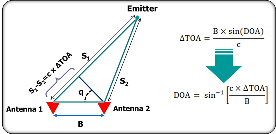
Figure 1: DTOA Technique principle of operation
In a dual channel ESM featuring a short base length B, compared with emitter range R, the difference in TOAs provides Direction Finding: the DF accuracy is proportional to the antennas base length.
The TDOA Technique strongly depends on:
- Distance between radiating elements
- Time unbalances between Rx channels
- Variations in time of the received signal used to establish arrival time differences
- Installation (due to the impact of nearby reflections)
Basic assumptions
The Time comparison Technique does have some similarities to the Phase comparison one, but also some differences:
- as in the case of Phase comparison, TOA comparison Technique requires antennas having:
- same shape,
- parallel Bore-Sights [BS],
- given displacement;
- as in the case of Phase, the measurement from which is inferred the angular information is the path difference (even if in term of time delay instead of phase delay) between the wave-fronts arriving to different antennas;
- the main difference (as it will be clearer later) is that the TOA measurement is not ambiguous (as in case of the phase) so there is no need of multiple baselines.
- Another key difference is that the TOA techniques do not depend on the frequency (or at least they weakly depend on it)
So let us consider the simple 2-Antennas (namely “a” and “b”) system depicted in Figure 2 where is shown a wave-front – impinging the Antennas – having ![]() a angle w.r.t. the BS.
a angle w.r.t. the BS.
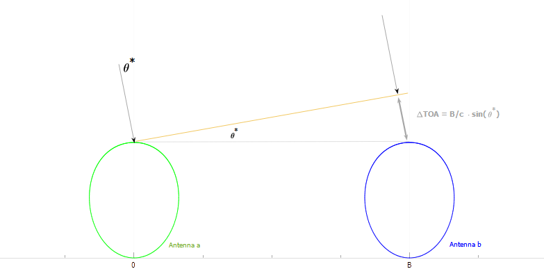
Figure 2: TOA Comparison Technique concept
If we assume the wave-front arriving at Antenna “a” at – say – ![]() , the same wave-front shall reach the Antenna “b” at
, the same wave-front shall reach the Antenna “b” at ![]() , being
, being ![]() the time needed to the light to cover the B
the time needed to the light to cover the B ![]() span:
span:
![]()
Where:
- B is the so called “baseline” (e.g. the spacing between the antennas).
- c is the speed-light, e.g.
 m/s.
m/s.
As it shall more evident in the following the “baseline” needed (in order to achieve acceptable performances) range from 5 to 15 meters.
Derivation of the Algorithm
DOA estimation is easily achieved as:
![]()
DOA Estimation Performance
In order to get the DOA estimator performance we can start form the following identity:
![]()
Then we can substitute as follows
![]()
Where:
 is the impairment onto the Time difference measurement
 is the induced DOA error
Finally we get:
![]()
Where:
 is the rms error which affects the TOA difference measurement
- The term
 represents the “DF slope” relating the TOA measurement accuracy to the wanted DF accuracy.
It has to be noted that – due to the ![]() dependency – a single DTOA baseline is typically used to cover no more than 120° (e.g. ± 120° w.r.t. the Bore-Sight).
dependency – a single DTOA baseline is typically used to cover no more than 120° (e.g. ± 120° w.r.t. the Bore-Sight).
System level considerations
Hereafter are reported some important considerations from the point f view of EW System design.
- Signal Parameter
- The time measurement is the more critical aspect of the Technique: since accuracies in the order of a few nanoseconds have to be reached.
- Fine digital processing algorithms are often used in modern EW System using digital receivers, which combine fast ADC’s and interpolation techniques.
- Difference of TOA measurements – which are intrinsically related not only on the performance of the receiving system – but are also related to the intrinsic properties of the incoming signal are usually well suited in case of Radar signals which usually exhibits wide bandwidths.
- Requirements/Issues on the EW System.
- Number of Antennas:
-
- The number of Antennas is typically
-
- 4 Antennas (when a full 360° is required).
- 2 Antennas (when – as typical of airborne application – a ‘side-looking’ of say ~ 120° is required).
- Number of DF Channels:
-
- At least two channels are required.
- In case of EW Systems involving 4 Antennas the 2 Channels could be switched between all possible couples of antennas.
- Calibration:
-
- Time calibration – which is less demanding w.r.t. the Phase one – has to be carried out onto the analog part of the receiver.
- Synchronisation:
-
- Time synchronisation is an important factor to be taken into account.
- Since usually the TOA measurement operates on the Band-Width [BW] of the signal and not over its carrier, the synchronisation requirement is slightly less demanding than in case of Phase measurements.
- Kind of DF Channels:
-
- TOA comparison Techniques typically achieves the best performance with Super-Heterodyne [SH] channels having quite wide BW, the need for fine digital processing requires also the use of fast ADC’s.
- Typical DF performances
- Typical DF performances are shown in Table 1 for baselines equal to5, 10 and 15 meters assuming TOA accuracies in the order of a few nanoseconds
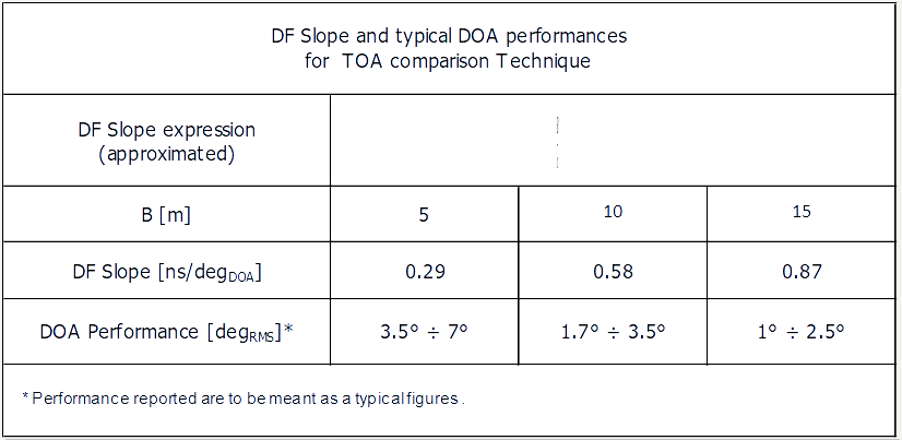
Table 1: Typical DF performances
- As it can be seen baselines in the order of ~ 10 m are needed for acceptable performances.
- Pros
- Time comparison Technique – thanks to the availability of fine processing capabilities in modern EW receivers – has become quite popular since it represents a good compromise between performance and complexity.
- Being – in theory – independent from the Frequency (this is a big difference w.r.t. the Phase comparison) the TOS comparison Technique does not need the partition of the System BW in some sub-Bands.
- “Impact on Platform”
- The main impact on the platform is the need for the Antenna’s distance which makes this Technique well suited for naval and wide-body airborne platforms.
Figure 3 shows an idealized example of aircraft installation of a DTOA goniometer.
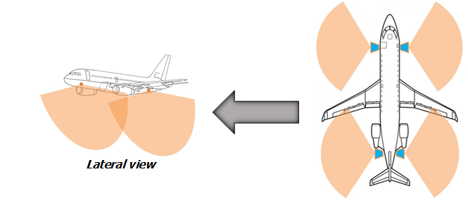
Figure 3: example of aircraft installation of a DTOA goniometer
Figure 4 shows the concept for the DTOA application covering the full 360° Azimuth and the study for the possible mast installation.
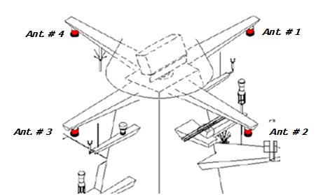
Figure 4: DTOA concept & installation (full 360° Azimuth coverage) for naval application