Passive Direction Finding [DF] Techniques – Phase Comparison

In an Phase Mono-pulse DF system (Phase-interferometry) more antennas (≥3) are arranged in different spatial positions to form an array to accurately estimate the direction of arrival of a signal from the phase difference of the signal measured on the array antennas.

The accuracy of the AoA estimate is proportional to the array baseline and to the phase unbalance between the two channels up to the final phase detectors.

Phase comparison is usually implemented with some panels (the so-called Interferometric Panel [PI]) each operating over say 180° Azimuth but covering actually a reduced sector (typically 120° intended as ± 60° w.r.t. the Bore-Sight)

In Phase comparison Technique, the Antennas are supposed:

• to have the same shape,
• to have parallel Bore-Sights [BS],
• to be displaced each other with given (and known) distances

The phase measurements are possible using the same phase detector architecture adopted for an IFM receiver, with a proper number of channels (one for each antenna of the array).

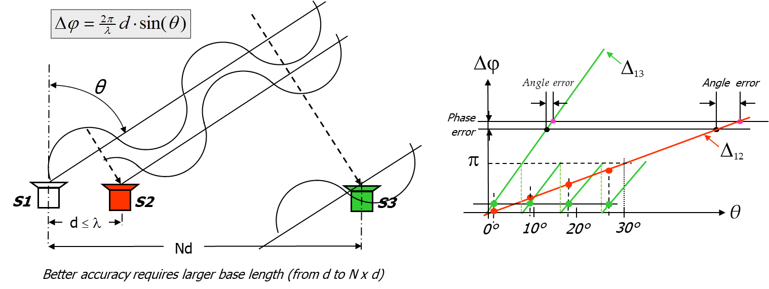
Figure 1: Phase comparison Technique concept

This solution features a very limited dynamic range (Figure 3).

A more modern solution employs a multichannel DRX, providing a larger instantaneous dynamic range, depending on the DRX number of bits.

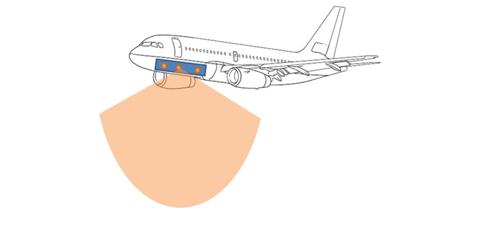
Figure 2: Example of side-looking interferometric panel

In both the above solutions a calibration procedure for each channel is mandatory to achieve the required phase accuracy.
Moreover a phase matched calibration matrix must be provided.

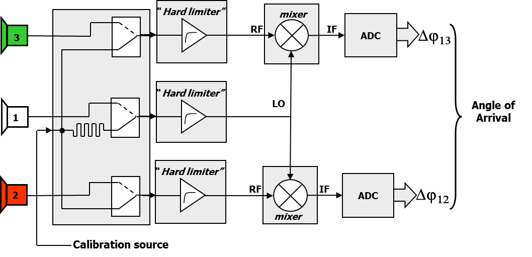
Figure 3: Example of phase comparison mono-pulse DF analog receiver

Basic assumptions

In order to introduce the main concepts of this Technique let us consider the simple 3-Antennas (namely “a”, “b” and “c”) system depicted in Figure 4 where is shown a wave-front – impinging the Antennas – having a angle w.r.t. the BS.

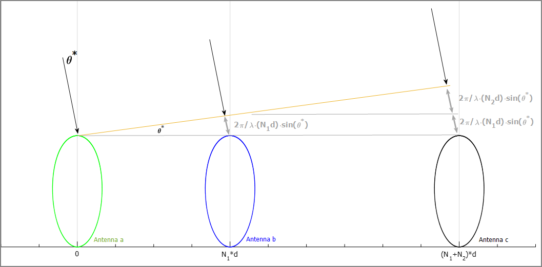
Figure 4: simple 3 antennas interferometric system

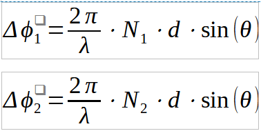
In what follows we shall assume that – as indicated in Figure 4 – the 2^nd Antenna is far from the 1^st Antenna and the 3^rd Antenna is far from the 2^nd one: the overall span is  . A 3-channel Receiver is also assumed, able to provide a measurement of the phase difference between Antenna “b” and Antenna “a” as much as the difference between Antenna “c” and Antenna “b”.

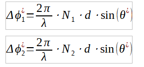
Now we must take into account that – even if previously equations are monotone functions of (when it is ranging from -90° up to +90°) – the actual phase difference values measured are modulo 360° reduced, as shown in Figure 5 (which also shows the “ambiguity indexes”, namely and ).

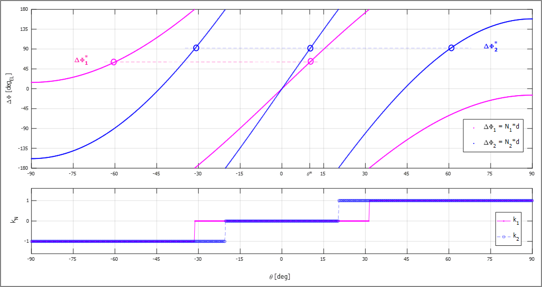
Figure 5: ΔΦ’s modulo 360° reduced and orders of ambiguity

Looking to Figure 5 we can observe that:

• there are more values of corresponding to the same value of ,
• there are more values of corresponding to the same values of ,
• there is only corresponding to both and   : this means that the two “interferometric baselines” herein proposed are jointly not-ambiguous.

Derivation of the Algorithm

In this section, we shall avoid mathematical details and we will limit ourselves to explain the basic concept of the so-called “ambiguity resolution” problem.

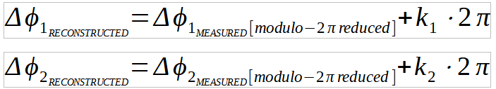
The ambiguity resolution consists in estimating the values of   and which are needed to make monodromic the values of Phase differences (which – as previously said – are measured as modulo-360°):

The ambiguity resolution is probably the major issue of the Phase comparison Techniques, in fact we have to follow 2 steps:

1. individuate the “interferometric baselines” which allow for a safe ambiguity resolution (see [1] which is a very good treatise on 2-base and 3-base Phase DF),
2. find out a good algorithm (e.g. having the best compromise between performance and complexity).

In order to understand how a resolution ambiguity algorithm work we propose Figure 6 in which is depicted the behaviour of the ambiguity indexes and (for the use case shown in Figure 4 and Figure 5) represented onto the – plane

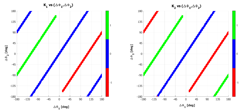
Figure 6 – k1 and k2 seen as a functions of (ΔΦ1, ΔΦ2)

From Figure 6 it is clear that – looking jointly to and – it is possible to find out the right values of  and. As an example let us assume that the receiver provides the following values:

• ~ -135°
• ~ +155°

According to Figure 6 the only values, which cope with these are:

• = 0
• = -1

Using previous we shall be able to find out the actual Phase difference values namely and .

Even if many systems composed by two (or more) interferometric baselines can be thought, the basic principle of ambiguity resolution is the same we presented. Methods used to solve the ambiguity can be based onto:

• Analytical resolution of the boundary in the ΔΦ’s space,
• Tabulated functions (implemented using Look-Up Tables [LUT]),
• Hybrid approaches achieved by mixing the both.

Now we can use previously defined identities:

Adding the two above expression lead to:

Finally, the DOA estimate can be achieved as:

DOA Estimation Performance

DOA performance can be assessed starting from the above expressions under the assumptions that the ambiguity resolution was successful.

Starting from:

We can put:

Where:

• is the error on the DF estimate,
• represents the ensemble of all impairments on the Phase difference measurement.

We can use the simple Taylor Series development in order to get:

Where:

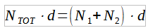• is the overall length available for the Interferometric Bases
• represents the generic k^th impairment.

As it can be seen in the previous expression, the performance exhibits a strong dependency upon the Frequency, being : in Figure 7 is depicted a typical behaviour vs Frequency over a Band-Width [BW] ranging from f_MIN to f_MAX.

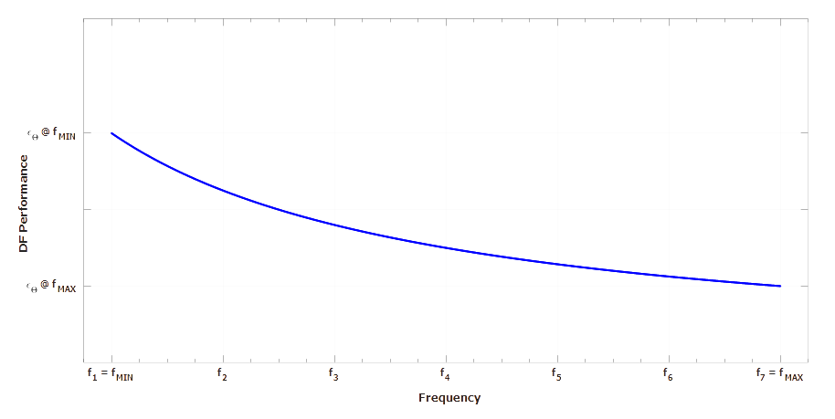
Figure 7 – Typical behaviour of the DF performance over a wide BW.

System level considerations

Below we report some considerations about the systemic use of the technique.

• Signal Parameter

• Since DOA estimation is inferred through the Phase difference between (at least) three Antennas a Receiver able to measure the phase must be used
• The Frequency also is a fundamental parameter to be estimated in order to
  • Estimate the wave-length λ
  • Provide a tight calibration
• The importance of the Phase also lies in the fact that it is more robust than the Amplitude w.r.t. environmental effects (e.g. multipath), however we have to consider that receivers able to measure the Phase are, generally speaking, a little bit more complicated than receivers able to measure the Amplitude.

• Requirements/Issues on the EW System.

• Number of Antennas:

• The number of Antennas is a key parameter since we have to take in to account for:

• • Ambiguity solving, which requires at least three antennas for a single PI.
  • Achieving the performance over a wide BW, which could require the partition of the whole BW in some sub-Bands (each having its own PI).
  • Azimuth coverage, as previously indicated a single PI could cope with a sector of, typically, 120° (e.g. ± 60° w.r.t. the Bore-Sight of the PI).

• Number of DF Channels:

• • • • The number of Channels is still an important factor: due to the need to measure simultaneously all Phases on each Antenna (in the same PI) the number of channels must be at least equal to number of antennas within the PI.
      • In order to reduce the amount of the whole hard-ware a single set of channels could be switched between different PIs.

• Calibration:

• Phase comparison is probably the most demanding Technique from the point of view of Calibration: since also slight differences between Gonio channels could lead to not negligible phase impairments, a tight calibration mechanism has to be designed.

• Synchronisation:

• Synchronisation is also another critical aspect which has become always more important with modern Digital Receivers in which the back-end of Gonio Channels is digitized.

• Kind of DF Channels:
  • As indicated above the EW System must be equipped with receivers able to provide the measure of the phase.
  • Previous receivers used analog phase comparators or phase detectors.
  • Modern receivers use Super-Heterodyne [SH] receiving channels, sometimes coupled with ADC in order to perform measurements with the aid of signal processing: both I/Q or IF digitizers are used.

• Typical DF performances

• Phase comparison is perhaps the most effective Technique for achieving the best performances.
• In Table 1 are shown some typical performance: obviously, the real achievable performance strongly depends upon the actual phase impairment that can be reached.

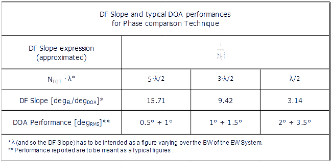
Table 1 – Typical DF performances

• What is important to understand is that the technique is very dependent on frequency so one of the most significant trade-off to be done is the choice regarding the number of sub-Bands partitioning the whole BW.
• A further important trade-off is that one regarding the Phase DF Slope: in fact the higher the DF Slope, the better the performance but also the greater the ambiguity level.

• Pros

• The most attractive feature of the Phase comparison Techniques are:

• • The higher robustness of signal Phase w.r.t. other parameters.
  • The opportunity to get very good performances.

• “Impact on Platform”

• as already mentioned, the greatest impact on the platform is probably due to the fact that you do not have to install single antennas but PI unit.
• Typical application of the Phase comparison Technique are:

• • EW Systems covering the full 360° Azimuth in naval and ground platforms.
  • PI units covering ~ 120° (the so called ‘side looking’ mode) for airborne applications.

Below some example of Interferometric DF installation, both in the sea and air case.

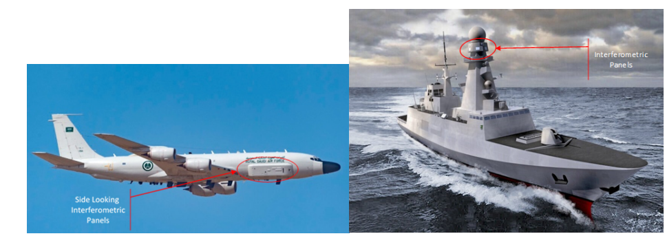
Figure 8: examples of installation of interferometric panels in airborne and naval platforms