De-interleaving process in RESM

The receiver sends the information to the De-interleaving Process in the form of digital message called PDM (Pulse Descriptor Message).
This message is the EME representation in terms of measures of RF, DOA, PW, plus other information that the receiver is able to measure (e.g. Intra-pulse modulations and eventually its characteristics, measure validity, etc…)

Therefore the PDMs (Pulse Descriptor Messages) that enter the De-interleaver are a confused mix of signals belonging to several emitters that can also present characteristics of agility in time and frequency that can further complicate their classification.

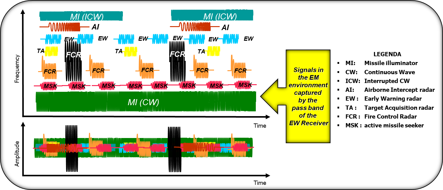
Figure 1: Example of EW Scenario

The output of the De-interleaving Process are Radar tracks (or Radar emitters) and their characteristics (PRI, PRI modes, RF, RF modes, PW, DOA, etc…) and feeds the Active Track File (ATF).

Therefore the task of the De-interleaver is to extract pulse trains of a single emitter starting from samples of digitized radar pulses, PDM’s measured and ordered in previous chains according to a set of rules called “Taxonomy” which collects the various types of notations and therefore describes the way in which the de-interleaving process “knows” the Radars in the EM Environment.

The main purpose of the de-interleaving is to separate signals that are ambiguous in frequency and angle of arrival and to calculate the PRI.

The De-interleaver can be therefore described by an n-dimensional function having as input a series of parameters characterizing the pulses and as output an emitter as unambiguous as possible in the space of possible emitters.

The De-interleaver is composed by firmware and software processes that extract emitters during a number stages, as follows:

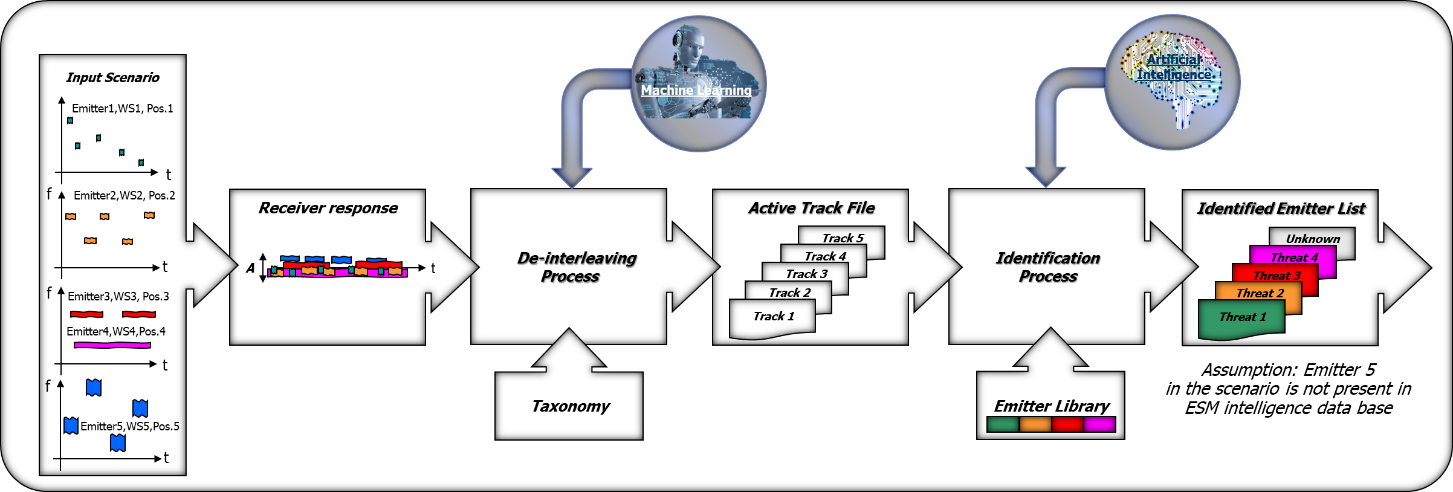
Figure 2: De-interleaving in the RESM value chain and its evolution

Firmware process: Clustering.

Clustering being a very fast process needs to be carried out in FW, it carries out the channelling of the PDMS in “chains” (substantially sub-sets of PDMs), the chains are structured with comparators in order to collect PDMs whose parameters (e.g. RF, PW and DOA) fall within pre-defined ranges.

The chains can basically be of three types depending on the criterion used for the association:

1. Unknown emitters (not already received and classified): the first “new” PDM that arrives (not compatible with the header of any other channel) creates a new “pulse chain” by “opening” a new channel configured with its own parameters.
2. Emitters already received: to reduce the processing load and the memory occupation space, channels can be defined with parameters derived from the tracks already present in the “Active Track File” and therefore take into account the knowledge of the electromagnetic scenario already acquired (scenario learning).
   The chains in these channels, being confirmatory and not discovery chains, require the storage of a smaller number of PDMs.
3. Emitters defined in the “Library”: if there is a need to manage alarming threats, “fast” channels can be defined which have parameters dictated by the Warning Emitters present in the Library and whose immediate channelling is required (the flag “alarm” present in the Library item asks for forced channelling at the beginning of the clustering process).
   The presence of this type of channels simplifies and accelerates the extraction of emitters deemed dangerous (threats) and therefore deserving of a” preferential lane “.
   The presence of this type of chains is linked to the concept of de-interleaving based on a-priori knowledge of the expected scenario and is defined in the MDP (Mission Data Package).

Clustering operates a real partition of PDMs: that is, each PDM can “enter” only one chain (i.e. the first whose parameters are adapted to that PDM).

The Clustering output is the “Radar Mode” which represents one of the many behaviours or operating modes of a Radar (an Emitter or Track representative of a Radar can have many Radar Modes).

Software process is divided in several modules, two of them are service modules:

• The Data Manager module organizes the data format to make the de-interleaving process receiver agnostic (PDMs can have formats that vary depending on the System), it acts as the interface between the Clustering and the following Processes.
• The Time Analyser module is a module that manages the memory occupation and the computation load: it has both monitoring and “run time” optimization purposes, it acts as the manager of the following Processes trying to increase the overall efficiency.

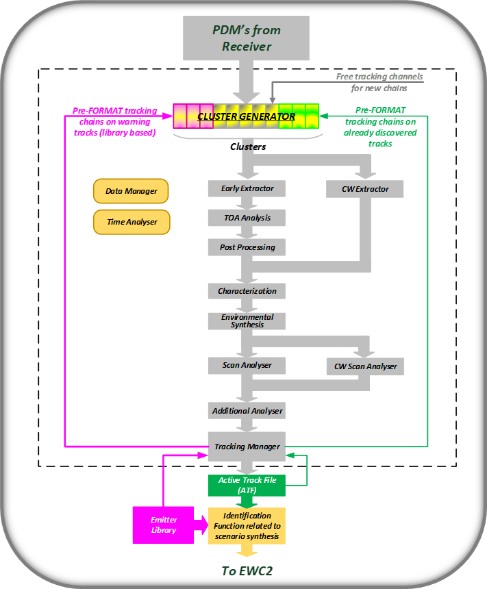
Figure 3: de- interleaving flow diagram

The other are operational modules:

• The CW Extractor module is dedicated to the extraction of the CW: the CW emitters deserve an “ad hoc” treatment since, not being impulsive, they require not only a dedicated analysis but also a treatment strictly linked to that performed by the Rx on CW signals (personalized module).
• The Early Extractor module is the module that operates on impulsive emitters and carries out the “TOA analysis” that is carried out on each chain and includes:
  • Creating Histograms: associate PRI values ​​and PRI templates.
  • Auto-correlation: finds pulse trains using the PRI values ​​provided by the histograms.
  • Adaptive Window: (AW): if auto-correlation cannot find a pulse train, a process starting with 2 pulses is used, their TOA delta gives the probable PRI, then looks for the next pulse within of an interval of an acceptance window.
    The algorithm includes a mechanism whereby the window is continuously adapted based on the jitter shown by the pulse train.

The lost impulses are separated and accumulated in a bin as “waste” which are analysed again at the end of the whole process to find more “exotic” matches, this module works “serially” chain by chain.

• The Post Processing module verifies whether different simple Radar Modes can belong to a complex Emitter and in this case associates them in a single Emitter, as an Emitter can be formed by one or more Radar Modes (multi-mode or multi-functional radar).
  

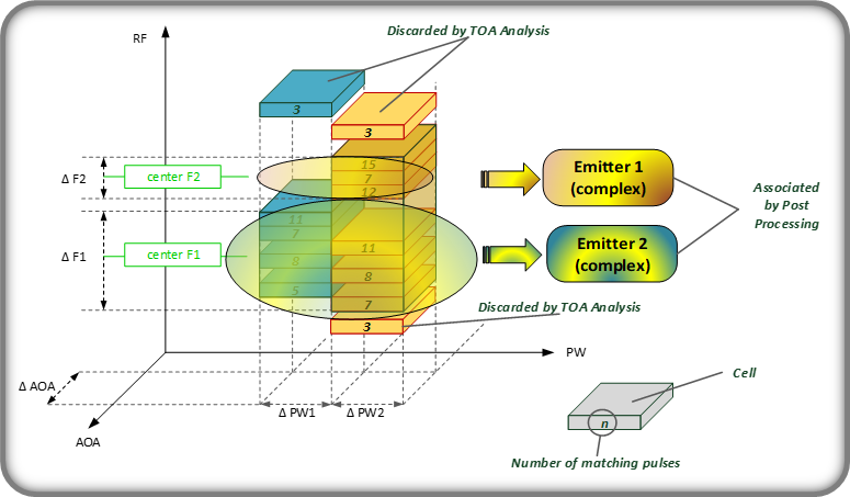
Figure 4: complex emitters re-construction

• The Characterization module works in strict conjunction with the previous one and identifies the notations and the characteristic values ​​in the RF and PW domain and provides an estimate of the DOA (by integrating values coming from the collapsing of several radar modes into a single emitter), also this module works “serially” chain by chain.
• The Environmental Synthesis module checks the compatibility of what is extracted in the current “Frame” with the pre-existing “Track File” in order to decide whether to update Tracks already present and or to create new Tracks in the Active Track File (ATF).
• The Scan Analyser and CW Scan Analyser modules (long term analysis) perform scan analysis: they are differentiated in that the CW Emitters, unlike the Impulsive ones which are easily generalizable, require customization on the specific System because the related PDMs are strongly dependent on the type of Rx; this module also works “serially” chain by chain;
• The Additional Analyser module carries out checks and additional estimates on ancillary parameters (e.g. spurious, MOP parameters) this module also works “serially” chain by chain;
• Finally, the Tracking Manager module is dedicated to setting up the Clustering (manages the header of type 2 and 3 chains) and closes the loop between the SW part and the FW part of the whole Process.

The outcome information is then compared with the emitter library for a match and the resultant data is logged in the Active Track File (ATF).

The active Track File maintains a list of active emitters, evolving for the duration of mission, it is the central database of the ESM and contains information of all parameters measured and peculiar characteristics of each emitter intercepted by the system in a given period of time.

Taxonomy

Radar Emitters are modelled in terms of “Radar Mode” (in general, each Radar can have multiple Modes) and a Radar Mode is defined based on its fundamental parameters (RF, PW and PRI) both in terms of values ​​and notations:

• The values ​​are numeric data that express the interval to which a parameter belongs.

• The notations summarize the evolution process of that parameter in the domains of time, frequency and amplitude.

Taxonomy is a set of rules embedded in the de-interleaving process itself that tries to give a standard definition to all the forms in which a radar can be intercepted, made up with the collection of the various types of radar notation and therefore defining how the de-interleaving process “knows” the radar.
Taxonomy can also be interpreted as a sort of “default library” that is not a function of the type of the system in which it resides or the type of mission that must be carried out.
The concept of Taxonomy is fundamental to understand the functioning of the de-interleaving process, in fact, it must be clear that the de-interleaving process will synthesize not the Radar Emitters actually present in the EM environment but the Emitters which, in function of the collected data (e.g. PDM), are compatible with the Taxonomy.

The Taxonomy is defined on the basis of experience in order to be as representative as possible of the “Radar world”, however, it must be clear that a Radar, unlike a generic Radio Communication System (which operates on the basis of a standard that defines the waveforms, protocols, strategies to access the EM medium, etc.), has no necessity to obey any standard.
Each Radar, therefore, while responding to what are the typical “guidelines”, potentially represents a “case in itself” and the Taxonomy that aims to “generalize” the Radar Emitters certainly cannot take into account the particularities and peculiarities of each Radar.

For this reason, the Taxonomy is used as a guideline for the de-interleaving process, while for the more accurate identification process the “Emitter Library” is used, part of the MDP (Mission data Package), which has a much more accurate genesis, being derived from intelligence data and adapted mission by mission.

The Library, as we have already seen previously, has interactions with the de-interleaving process in the following two ways:

• at the Clustering level: “prioritizing” and defining the input parameters of specific Clustering chains (and therefore allowing the prior selection of the PDMs pertaining to the Emitters present in the Library with a sort of “preferential lane”); it is also possible to associate the temporal parameters (notation and PRI values) of the Emitters present in the Library to the pre-headed chains on a library basis in order to further drive the synthesis of the same Emitters.
• at the level of “Environmental Synthesis”: essentially it is as if the Library were to somehow increase the Taxonomy and allow the association of Emitters, making use of “a priori” information, which otherwise would not be collapsed in a single Emitter by the de-interleaving process.

Future developments

Electronic Warfare in general is field in which Artificial Intelligence and Machine Learning can have a wide application.
This is the case of Radar De-interleaving, the process of separating several electromagnetic signals collected in the EM scenario and assessing to what RADARs they belong, that is traditionally performed via imperative algorithms.

However this approach has already reached its limits.
This is due to the fact traditional algorithms take into consideration one domain, like Time, RF, DOA, Pulse Width, at a time which eventually provides poor performances when dealing with actual complex and contested EM environments with several missing pulses.
In fact, the environment is typically very dense and composed of RADAR instances potentially similar to each other in terms of Frequency, PRI and PW.
Additionally, modern multifunctional RADARs are difficult to be framed in any existing taxonomy since they lack of pulse periodicity (or PRI agility), which is typical of older RADARs.

This pressing issue is opening the door to the use of deep learning to electromagnetic signal classification for EW applications.

A novel de-interleaving approach based on neural networks (like Convolutional Neural Network and Deep Learning approaches in general) could instead consider all the aforementioned domain at the same time exactly as an ELINT Operator would do.
A different kind of neural network like Recurrent Neural Network (i.e. Long Short Tem Memory, LSTM) could be trained in order to consider the past sequence of n pulses and assess whether the n+1 is compatible with them or not.
Such instantaneous multi domains and sequence dependent approaches can be combined via model stacking in order to exploit and combine their benefits.

The real issue, is the availability of data needed to train the A.I. based engines whatever the branch of A.I. we want to apply and this imposes methods and procedures at User level for the success of the enterprise.

This will be the matter of a novel discipline named Cognitive EW in the two branches of Cognitive Texture Classification and Cognitive Event Classification.